04: Bringing it together
Contents
%matplotlib inline
from matplotlib import pyplot as plt
from IPython.display import YouTubeVideo
import qutip
import numpy as np
import naq
04: Bringing it together#
Schrödinger equation#
The Schrödinger equation gives the evolution of a state \( \psi \) as a function of time, \( t \).
We also need an initial state to start the evolution from, usually called \( \psi_0 \) or \( \rho_0 \).
QuTiP provides a handy function, sesolve, for solving this for a given
Hamiltonian, \( H \).
In general, the Hamiltonan may also be a function of time, \( t \), so that the Schrödinger equation becomes:
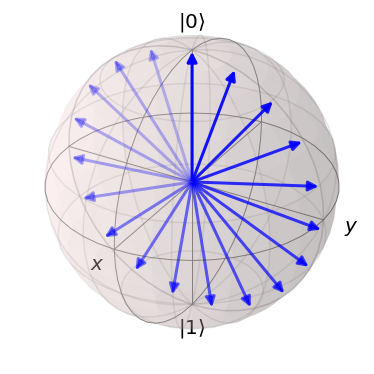
Let’s try out sesolve:
SX = qutip.sigmax()  # rotate around the X axis in time
g = np.pi / 10  # rotate 1/10 of pi per unit time
H = g * SX

psi0 = qutip.basis(2, 0)  # start in the first basis state
tlist = np.linspace(0, 10, 20)
result = qutip.sesolve(H, psi0, tlist=tlist)

bloch = qutip.Bloch()
bloch.vector_color = ["b"] * len(result.states)
for i, s in enumerate(result.states):
    bloch.add_states([s], alpha=0.2 + 0.8 * (i / len(result.states)))
bloch.show()

The sesolve function takes a few other options:
e_ops: a list of measurement operators for storing expected outcomes of measurements of the state instead of (or in addition to) the states themselves.options: an instance ofqutip.Optionsthat allows one to change the behaviour of the underlying ODE integrator. An important option isnstepswhich specifies the maximum number of internal steps the integrator should take between times intlist.
For example, if one has a rapidly evolving system, one might need to
drastically increase nsteps, e.g.:
options = qutip.Options(nsteps=200_000)
result = qutip.sesolve(H, psi, tlist=tlist, options=options)
Density matrices#
So far we have dealt with “pure” quantum states, i.e., descriptions of quantum systems that are in a specific quantum state.
Density matrices capture the concept of an ensemble of states, i.e., a situation where we have only probabilistic knowledge of which “pure” state the system is in.
Note that this is different from a superposition of states.
Pure states may already be superpositions. Superpositions are combinations of pure states that combine to give another pure state. The coefficients are amplitudes – i.e. complex numbers. The squares of the lengths of the amplitudes must sum to 1.
Ensemble states are also combintations of pure states, but the coefficients are probabilities – i.e. real numbers. The probabilities (not their squares!) must sum to 1.
Density matrices are ubiquitious in quantum mechanics because when on asks oneself what the state of a sub-system of a bigger system is, the answer is in general only probabilistic – i.e. an ensemble of the states of the smaller system.
A density matrix is represented as an opertor – i.e. a function that maps states to other states. All density matrices may be written in the form:
For a pure state, \( \psi \), the corresponding density matrix has the simple form:
For a pure state there is only one state in the ensemble, \( \psi \) and its probability, \(p_{\psi}\), is \( 1 \).
In QuTiP we can write this as:
psi = qutip.basis(2, 0)
rho = psi * psi.dag()
print(rho)
Quantum object: dims = [[2], [2]], shape = (2, 2), type = oper, isherm = True
Qobj data =
[[1. 0.]
 [0. 0.]]
or use the built-in function, ket2dm:
psi = qutip.basis(2, 0)
rho = qutip.ket2dm(psi)
print(rho)
Quantum object: dims = [[2], [2]], shape = (2, 2), type = oper, isherm = True
Qobj data =
[[1. 0.]
 [0. 0.]]
Rydberg Blockade#
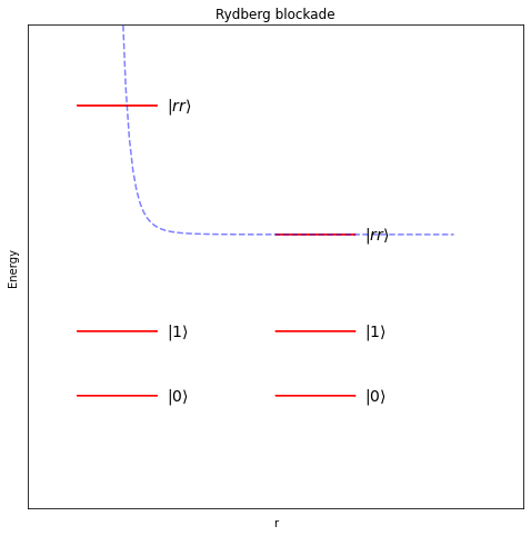
A reminder of the Rydberg blockage mechanism:


