03: Describing a qubit
Contents
%matplotlib inline
from matplotlib import pyplot as plt
from IPython.display import YouTubeVideo
import qutip
import numpy as np
import naq
03: Describing a qubit#
Building quantum states#
Let’s review our two basis states:
# Our two basis states:
b0 = qutip.basis(2, 0)  # 6s
b1 = qutip.basis(2, 1)  # 7s
When writing these mathematically we write \(\left\vert 0 \right\rangle\) and \(\left\vert 1 \right\rangle\).
The states b0 and b1 are instances of Qobj, which qutip uses to
represent all sorts of quantum objects.
Let’s take a closer look at b0:
print(b0)
Quantum object: dims = [[2], [1]], shape = (2, 1), type = ket
Qobj data =
[[1.]
 [0.]]
The Qobj data is the array that represents our quantum state. As you can
see, it’s just a column vector:
The shape is just the shape of the data – i.e. (2, 1).
The type says this is a ket which is the strange word physicists use to
say that it is a quantum state.
The word dims is short for dimensions. It describes how the state is built
up from smaller states. Since our state has no smaller states, it currently
looks identical to the shape. We’ll look at this again when we add more
atoms later on.
You can also access this informaton using attributes:
print(b0.type)
print(b0.shape)
print(b0.dims)
ket
(2, 1)
[[2], [1]]
If we look at b1:
print(b1)
Quantum object: dims = [[2], [1]], shape = (2, 1), type = ket
Qobj data =
[[0.]
 [1.]]
It’s just the column vector:
If you’re familiar with vector spaces, you’ll already recognize these two column vectors as basis vectors, and indeed the space of quantum state will be a vector space.
The other states that can be built from our two basis states are:
where \(a_0\) and \(b_0\) are any two complex numbers.
These two numbers are called amplitudes. For our particular basis they have
the interpretation that if we measure the energy of the state
\(\left\vert \psi \right\rangle\) there is a probability \(|a_0|^2\) that the
energy measured will be the energy of the state b0 (i.e. the energy of the
electron in state 6s) and a probability \(|a_1|^2\) that the energy measured
will be the energy of the state b1 (i.e. the energy of the electron in
state 7s).
This association of amplitudes with probabilities is called “Born’s Rule”
and is one of the axioms of quantum mechanics (albeit one which many people
would like to remove).
Since the probabilities should sum to one, we have the constraint that \(|a_0|^2 + |a_1|^2 = 1\).
The value \(|a_0|^2 + |a_1|^2\) is the length of the vector squared, so the constraint is that the length of the vector describing the state should be 1.
We can construct these in qutip in exactly the way you would expect. Let’s construct some more ourselves:
print(1j * b0)
print(b0 + b1)
print(b0 - b1)
print(b0 - 1j * b1)
Quantum object: dims = [[2], [1]], shape = (2, 1), type = ket
Qobj data =
[[0.+1.j]
 [0.+0.j]]
Quantum object: dims = [[2], [1]], shape = (2, 1), type = ket
Qobj data =
[[1.]
 [1.]]
Quantum object: dims = [[2], [1]], shape = (2, 1), type = ket
Qobj data =
[[ 1.]
 [-1.]]
Quantum object: dims = [[2], [1]], shape = (2, 1), type = ket
Qobj data =
[[1.+0.j]
 [0.-1.j]]
You’ll notice that these vectors no longer have length one. In fact they have length \(\sqrt{2}\). This is no good. QuTiP has some functions to help.
The method .norm() returns the length:
psi = b0 + b1
print(psi.norm())  # prints the length
print(1 / psi.norm())  # prints the inverse of the length
1.4142135623730951
0.7071067811865475
And the method .unit() divides a state by it’s length, returning a new
state of length 1:
psi_unit = psi.unit()  # divide a vector by it's length, so that it ends u
print(psi_unit)
print(f"Length: {psi_unit.norm()}")
Quantum object: dims = [[2], [1]], shape = (2, 1), type = ket
Qobj data =
[[0.70710678]
 [0.70710678]]
Length: 0.9999999999999999
There is also another way that we write the length:
print(f"Length squared: {psi.dag() * psi}")
Length squared: Quantum object: dims = [[1], [1]], shape = (1, 1), type = bra
Qobj data =
[[2.]]
Let’s look at b0.dag() and (1j * b0).dag():
print(b0.dag())
print((1j * b0).dag())
Quantum object: dims = [[1], [2]], shape = (1, 2), type = bra
Qobj data =
[[1. 0.]]
Quantum object: dims = [[1], [2]], shape = (1, 2), type = bra
Qobj data =
[[0.-1.j 0.+0.j]]
We see that b0.dag() is just the transpose of b0. It’s shape is (1, 2)
and the dimensions are also swapped. It’s type is bra which is the
physicist way of saying it is a row vector.
However (1j * b0).dag() is a bit different. It’s the transpose, but the
imaginary part also has an minus sign in front of it. This is called
the complex conjugate.
So .dag() transposes the vector and applies the complex conjugate to each
element. Mathematicians call this the adjoint.
In mathematical notation we write \( {\left\vert \psi \right\rangle}^{\dagger} \) as \( \left\langle \psi \right\vert \).
where \( \alpha^{*} = (a + i b)^{*} = a - i b \).
Now when we multiply the the adjoint of a state by the state itself, we get an expression called the “inner product” that we can write as:
in QuTiP:
b0.dag() * b0as vector multiplication: \( \begin{bmatrix} \alpha^{*} & \beta^{*} \end{bmatrix} \begin{bmatrix} \alpha \\ \beta \end{bmatrix} \)
by just multiplying everything out: \( a^* a + b^* b = |a|^2 + |b|^2 \)
how physicists write it: \( \left\langle \psi \vert \psi \right\rangle \)
The “inner product” is also called a “bra-ket” (a bracket) because of the way
it is written. The bra (the adjoint of a state) is the left part of the
bracket and the ket (a state) is the right part. It’s a bit silly, but
very useful in practice.
Note that b0 * b0.dag() (a ket-bra) is something completely different!
ket_bra = b0 * b0.dag()
print(ket_bra)
Quantum object: dims = [[2], [2]], shape = (2, 2), type = oper, isherm = True
Qobj data =
[[1. 0.]
 [0. 0.]]
It has shape (2, 2) and dimensions [[2], [2]] and is of type oper which
is short for operator. As you can see, this one is a two by two matrix –
i.e. it transforms one state into another.
There is one final wrinkle in how the states are structured. In quantum mechanics, the values we can measure depend on the magnitude of the amplitudes, i.e. \( \alpha \) and \( \beta \), but only on the differences between phases of the amplitudes.
This means that if two states are related by being multiplied by \( e^{i \theta} \) for some angle \( \theta \), so that \( \psi_1 = e^{i \theta} \psi_2 \), then \( \psi_1 \) and \( \psi_2 \) are indistinguishable states. That is, they are really the same state!
When working with states, QuTiP and physicists both typically ignore this while doing calculations. They don’t try to ensure that the same state always has the same \( \alpha \) and \( \beta \). Instead they remember that only the differences of the phases are measurable, and are careful about checking whether two states are the same.
For example:
b0_phase = np.exp(1j * np.pi / 5) * b0
print(b0_phase)
print(f"Equal: {b0 == b0_phase}")
Quantum object: dims = [[2], [1]], shape = (2, 1), type = ket
Qobj data =
[[0.80901699+0.58778525j]
 [0.        +0.j        ]]
Equal: False
So the default equality check treats these as different states. To test whether two states are the same state, we use the inner product of the two states, which is only equal to one if the objects represent the same physical state.
print(b0.dag() * b0_phase)
print(b0.overlap(b0_phase))
Quantum object: dims = [[1], [1]], shape = (1, 1), type = bra
Qobj data =
[[0.80901699+0.58778525j]]
(0.8090169943749475+0.5877852522924731j)
The .overlap() method calculates the inner product of the two states,
i.e., \( \left\langle \psi_1 \vert \psi_2 \right\rangle \).
There is also a great way to visualize states made from two basis elements which we will cover next.
Bloch sphere#
We can write any state made from two basis states as:
but we still need to introduce the constraint \( |\alpha|^2 + |\beta|^2 = 1\) and ensure that we used only the difference in phase between \( \alpha \) and \( \beta \).
We can satisfy the first constraint by recognising it as requiring that the magnitudes of \( \alpha \) and \( \beta \) lie on a circle and writing them as the sine and cosine of the angle around the circle:
Now if we write the difference in phase between \( \alpha \) and \( \beta \) as \(e^{i \phi}\), then we can write \( \psi \) as:
These two angles \( \theta \) and \( \phi \) can be interpreted as spherical the spherical coordinates of the points of a sphere!
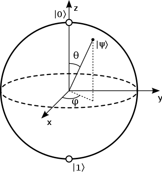
Fig. 4 How the angles \( \theta \) and \( \phi \) relate to the Bloch sphere.#
This representation of the space of all states made from two basis elements is called the Bloch sphere.
We can draw it in QuTiP like so:
bloch = qutip.Bloch()
bloch.vector_color = ["r", "b"]
bloch.add_states([b0, b1])
bloch.show()
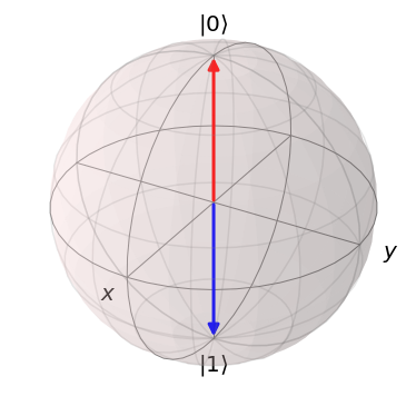
Note that our basis states b0 and b1 are the poles of the sphere,
which might be a bit unexpected since b0.dag() * b1 is 0. If we
were to consider the two vectors in 3D space, then b0.dag() * b1 would
equal -1.
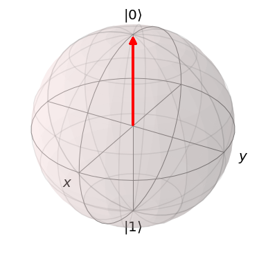
Let’s check that if we change the overall phase of a state, it doesn’t change where the state appears on the Bloch sphere:
thetas = np.linspace(0, 2 * np.pi, 16)
states = [np.exp(1j * theta) * b0 for theta in thetas]

bloch = qutip.Bloch()
bloch.vector_color = ["r"]
bloch.add_states(states)
bloch.show()
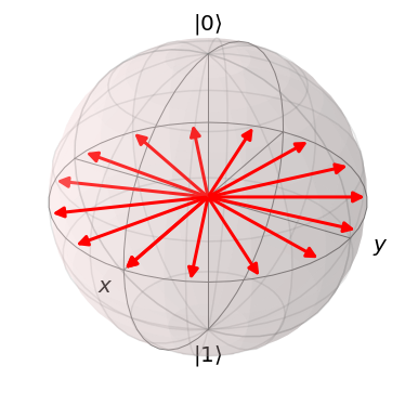
But if we change the relative phase, then the states are different:
thetas = np.linspace(0, 2 * np.pi, 16)
states = [
  (np.exp(1j * theta) * b0 + b1).unit()
  for theta in thetas
]

bloch = qutip.Bloch()
bloch.vector_color = ["r"]
bloch.add_states(states)
bloch.show()
