00: Introduction to QuTiP
Contents
00: Introduction to QuTiP#
In this first tutorial, you’ll play around with the core of QuTiP.
This includes constructing quantum states (e.g. qubits), quantum operators (e.g. gates in a quantum circuit), Hamiltonians, and density matrices. Near the end you’ll simulate the evolution of a quantum system using QuTiP’s numerical solver for the Schrödinger equation and visualize the result. Along the way you’ll find eigenvalues and eigenvectors and plot states on the Bloch sphere.
Individually none of the tasks should require more than a few lines of code, but there is a lot to explore. Take your time. Tackle individual steps in multiple ways. Read the documentation on the functions you’re using. Explore the objects you’re creating. Ask questions.
The topics covered in this tutorial will form the foundation we use during the rest of the week – and that you’ll use when using QuTiP yourself once the Summer school is over.
Tasks#
Pre-flight check#
If you haven’t installed Python, QuTiP, Jupyter and the other requirements yet, do so now by following one of the sets of instructions.
You can test that your setup is working by running the smoke test notebook.
Imports#
%matplotlib inline
import matplotlib.pyplot as plt
import qutip
import numpy as np
Helper functions#
def display_list(a, title=None):
    """ Display a list of items using Jupyter's display function. """
    if title:
        print(title)
        print("=" * len(title))
    for item in a:
        display(item)
def print_attrs(obj, name, attrs):
    """ Print the listed attributes of an object. """
    for attr in attrs:
        print(f"{name}.{attr}: {getattr(obj, attr)}")
def show_bloch(states, vector_color=None, vector_alpha=None):
    """ Show states or density matrices on the Bloch sphere. """
    bloch = qutip.Bloch()
    bloch.add_states(states)
    if vector_color is not None:
        if vector_color == "rb":
            vector_color = [
                (c, 0, 1 - c) for c in np.linspace(0.1, 1.0, len(states))
            ]
        bloch.vector_color = vector_color
    if vector_alpha is not None:
        bloch.vector_alpha = vector_alpha
    bloch.show()
def display_eigenstates(op):
    """ Display the eigenvalues and eigenstates of an operator. """
    evals, evecs = op.eigenstates()
    print("Eigenvalues:", evals)
    print()
    print("Eigenstates")
    print("===========")
    for v in evecs:
        display(v)
Accessing documentation#
Once you’re back home after the summer school, the QuTiP documentation will be your primary means of learning how to use QuTiP. In these tutorials, we’ll encourage you to read the documentation first, so that by the end of the week, you’ll be familiar with it and able to answer many of your own questions by reading it.
You’ll read the documentation in two main ways:
You can type a
?after any Python object to read its documentation. You can try it right now by typingqutip.ket?into notebook cell and pressing enter.You can find the documentation online at qutip.org. Open it now and have a look. You can also download it as a PDF in case you need to work offline.
States#
Creating and examining quantum states
Arithmetic with states
Checking whether states are equal and whether states with a different global phase are equal
What is a Qobj?
Functions you’ll want to try out in this section are:
qutip.ketqutip.braqutip.basis
These functions all return a “quantum object” or Qobj which is the data type QuTiP uses to store all kinds of quantum objects (states, operators, density matrices). A Qobj has some many methods and attributes that are useful.
Some attributes to look at include type, dims, shape, isket, and isbra.
A few important methods are .norm(), .unit(), .dag(), and .overlap(other).
You can use the arithmetic operators * and + as you would expect. Try out some simple numerical expressions from this morning’s theory lecture.
There are many more methods and attributes, but these are enough to start with.
# a qubit in the |0> state
ket = qutip.ket("0")
# show some of the properties relevant to kets
display(ket)
print_attrs(ket, "ket", ["type", "dims", "shape", "isket", "isbra"])
ket.type: ket
ket.dims: [[2], [1]]
ket.shape: (2, 1)
ket.isket: True
ket.isbra: False
# show the adjoint of the ket -- a bra
ket.dag()
# construct the bra directly
bra = qutip.bra("0")
# a qubit in the |1> state
qutip.ket("1")
# construct |0> and |1> using qutip.basis
q0 = qutip.basis(2, 0)
q1 = qutip.basis(2, 1)
display_list([q0, q1])
# show that Qobj's with the same values are equal
q0 == q0
True
# show that Qobj's with different global phases are not equal
display(q0 * 1j)
print("Equal:", q0 == q0 * 1j)
print("Overlap:", q0.overlap(q0 * 1j))
print("Overlap is 1:", np.abs(q0.overlap(q0 * 1j)) == 1.0)
Equal: False
Overlap: 1j
Overlap is 1: True
# orthogonal vectors have 0 overlap
q0.overlap(q1)
0j
# for states, the overlap is the inner product
print("q0 · q1:", (q0.dag() * q1).full()[0, 0])
print("q0 · q1:", (q1.dag() * q0).full()[0, 0])
print("(1j * q0) · q0:", ((1j * q0).dag() * q0).full()[0, 0])
q0 · q1: 0j
q0 · q1: 0j
(1j * q0) · q0: -1j
# adding states
q0 + q1
# calculating the norm
(q0 + q1).norm()
1.4142135623730951
# manually normalizing a state to unit length
(q0 + q1) / (q0 + q1).norm()
# using .unit() to normalize the length of a state
(q0 + q1).unit()
Bloch sphere#
Plotting 2-level states on the Bloch sphere
Plotting many states at once
Changing the colors
Changing the transparency
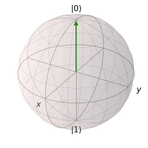
QuTiP provides a class called qutip.Bloch. You can create an instance of it and add states to plot with .add_states(...). Once you’ve added all the states you want to, you can all .show() to render it.
The Bloch sphere is very useful for visualizing the state of a two-level system, and you’ll use it regularly.
You can change the colors and transparency of the arrow shown for each state by setting the .vector_color attribute to a list of colors, and the .vector_alpha attribute to a list of transparency values.
# show a single state
show_bloch(q0)
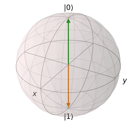
# show both basis states
show_bloch([q0, q1])

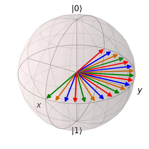
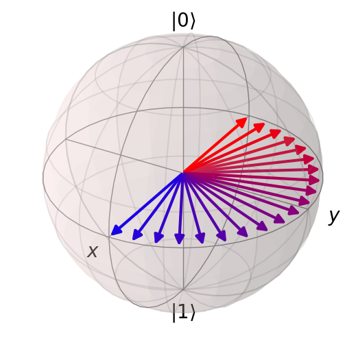
# show many states
theta = np.linspace(0, np.pi, 20)
states = [q0 + np.exp(1j * th) * q1 for th in theta]
states = [s.unit() for s in states]
show_bloch(states)
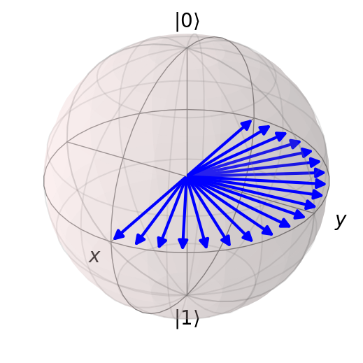
# How to remove the colours:
show_bloch(
    states,
    vector_color=[(0, 0, 1.0)] * len(states),
)
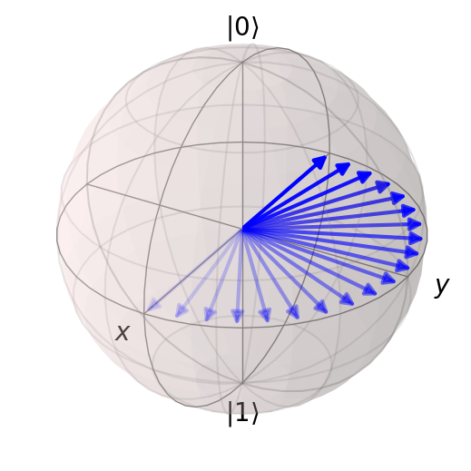
# Use transparency to show where states are in the list
show_bloch(
    states,
    vector_color=[(0, 0, 1.0)] * len(states),
    vector_alpha=np.linspace(0.1, 1.0, len(states)),
)
# Use color map to show where states are in the list
show_bloch(
    states,
    vector_color=[(c, 0, 1 - c) for c in np.linspace(0.1, 1.0, len(states))],
)
Operators#
Creating and examining quantum operators
Calculating expectation values
Making projectors
Functions to read about and try out in this section are:
qutip.sigmax,qutip.sigmay,qutip.sigmazqutip.qeyequtip.qip.operations.hadamard_transform
Operators are also represented by Qobj instances and there are some attitional Qobj attributes that are relevant now: type, isoper, dims, shape, isherm. Look at those you’ve seen already and compare them with what you’ve already seen for states.
There are some additional Qobj methods to try out on operators – .diag(), .tr() – and some to revisit – .dag(), .norm(), .unit().
You can create a projection operator by calling .proj() on a state. Try this out. Also try creating the projector yourself without calling .proj().
# the Pauli X operator
sx = qutip.sigmax()
# show some of the properties relevant to operators
display(sx)
print_attrs(sx, "sx", ["type", "isoper", "dims", "shape", "isherm"])
sx.type: oper
sx.isoper: True
sx.dims: [[2], [2]]
sx.shape: (2, 2)
sx.isherm: True
# show the adjoint
sx.dag()
# show the diagonal entries
sx.diag()
array([0., 0.])
# show the trace
sx.tr()
0.0
# show the (trace) norm
sx.norm()
2.0
# apply sx to the basis states -- it swaps them
display_list([sx * q0, sx * q1])
# construct the other Pauli matrices and the identity matrix
sy = qutip.sigmay()
sz = qutip.sigmaz()
I = qutip.qeye(2)
display_list([I, sx, sy, sz])
# Hadamard gate
H = qutip.qip.operations.hadamard_transform()
H
# Making projectors
q0.proj()
q0 * q0.dag()
Eigenvalues and eigenstates#
Eigenvalues
Eigenstates
It’s often important to know the eigenvalues and eigenstates of operators. QuTiP makes this easy. Read about and try out the .eigenenergies() and .eigenstates() methods of Qobj.
display_eigenstates(sz)
Eigenvalues: [-1.  1.]

Eigenstates
===========
display_eigenstates(sx)
Eigenvalues: [-1.  1.]

Eigenstates
===========
display_eigenstates(sy)
Eigenvalues: [-1.  1.]

Eigenstates
===========
Density matrices#
Creating density matrices
Plotting 2-level density matrices on the Bloch sphere
Plot some pure states
Plot some mixed states
QuTiP of course supports density matrices in addition to pure states. You can convert a state to a density matrix by calling qutip.ket2dm. You should also try construct some density matrices directly using the expression you saw in the theory lectures earlier.
One can also plot density matrices on the Bloch. Try it out! Once you’ve tried a few, attempt to predict how each density matrix will be represented before calling .show() and see if you are right. If you’re not right, read the Wikipedia article and try again.
rho0 = qutip.ket2dm(q0)
rho0
qutip.ket2dm(q0 * np.exp(0.1j))
q0 * q0.dag() # global phases cancel
rho = q0 * q0.dag() + q1 * q1.dag()
rho
rho.norm()
2.0
rho = rho.unit()
rho
bloch = qutip.Bloch()

bloch.add_states([qutip.ket2dm(q0), qutip.ket2dm(q1)])
bloch.add_states([rho])

bloch.show()
# p = 0.5 * (I + n . (sx, sy, sz))
# if p == 0.5 I, then n = (0, 0, 0)
rho == 0.5 * qutip.qeye(2)
True
basis = [qutip.qeye(2), sx, sy, sz]
for v in basis:
    display(v)
for v in basis:
    assert (v * v).tr() == 2.0
for v in basis:
    for w in basis:
        if v != w:
            assert (v * w).tr() == 0.0
Time-dependent operators#
Create a time-dependent operator
What is a QobjEvo?
Adding arguments
In QuTiP, time-dependent operators are represented by qutip.QobjEvo and not by Qobj. QobjEvo takes in a list of terms that are added together. Each term consists of a Qobj (the constant part) and a time-dependent coefficient function, like so:
sigmax_t = QobjEvo([[sx, "t"]])
Here sx is the operator and "t" is the time-dependent coefficient. Note that "t" is a string. QobjEvo turns this string into a very fast function for you. It’s also just very convenient to be able to write the coefficient function compactly.
Try out some other operators and some other coefficients, for example, "cos(t)" and "sin(t)".
You can evaluate a QobjEvo at a particular time by calling, for example, sigmax_t(2) or sigmax_t(0.1), or any other time. Create a state object that depends on time and plot its evolution on the Bloch sphere.
Lastly you can define coefficients that depend on arguments, such as "cos(w * t)". You need to supply an initial value for the arguments when creating the QobjEvo, like so:
sigmax_cos_t = QobjEvo([[sx, "cos(w * t)"]], args={"w": np.pi})
You can supply a different argument when calling the QobjEvo, for example, sigmax_cos_t(0.1, {"w": np.pi / 4}).
# Create a simple quantum object that represents sx * t
sigmax_t = qutip.QobjEvo([[sx, "t"]])
display(sigmax_t)
display_list([
    sigmax_t(t) for t in [0.0, 0.25, 0.5, 1.0]
])
<qutip.qobjevo.QobjEvo at 0x7f84888420e0>
# Multiplication:
display_list([
    (0.1 * sigmax_t)(1.0),
    (0.5 * sigmax_t)(1.0),
])
# Addition:
sigmay_t = qutip.QobjEvo([[sy, "t"]])
display_list([
    (sigmax_t * sigmay_t)(1.0),
])
# Take the conjugate and the adjoint:
display_list([
    sigmay_t.conj()(0.5),
    sigmay_t.dag()(0.5),
])
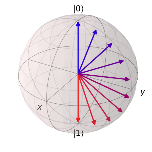
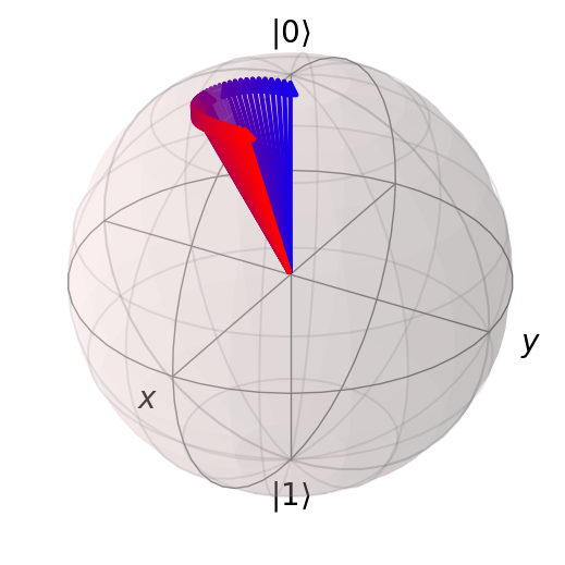
# Plotting the evolution under sigmax_t
states = [(1j * sigmax_t(t)).expm() * q0 for t in np.linspace(0, np.pi / 2, 10)]
show_bloch(states, vector_color="rb")
# Including a constant term
sz_plus_sy_t = qutip.QobjEvo([sz, [sy, "t"]])
display_list([
    sz_plus_sy_t(0.1),
    sz_plus_sy_t(1.0),
])
# Using a function like sin()
sz_sin_t = qutip.QobjEvo([[sz, "sin(t)"]])
display_list([
    sz_sin_t(t) for t in np.linspace(0, np.pi / 2, 4)
])
# Supplying arguments other than time
sz_g_sin_t = qutip.QobjEvo([[sz, "g * sin(t)"]], args={"g": 2.0})
display_list([
    sz_g_sin_t(np.pi / 2, args={"g" : g}) for g in [0, 0.2, 0.4]
])
Tensor products and partial traces#
Construct a state with two or three qubits
Construct an operator on multiple qubits
Construct an entangled state
Take the partial trace of a product state
Take the partial trace of an entangled state
QuTiP has two very useful methods for combining and separating sub-systems of a larger quantum state. Read about qutip.tensor and Qobj.ptrace and try them out.
q00 = qutip.tensor([q0, q0])
q00
pt_q0 = q00.ptrace(0)
pt_q0
q01 = qutip.tensor([q0, q1])
q01
display_list([
    q01.ptrace(0),
    q01.ptrace(1),
])
Hamiltonians#
Building Hamiltonians
Plotting eigenvalues
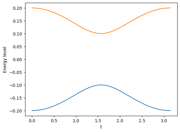
Now use everything you’ve learned so far to construct a time-dependent Hamiltonian and plot the evolution of its eigenvalues over time.
H = qutip.QobjEvo([[sx, "a * cos(t)"], [sy, "b * sin(t)"]], args={"a": 0.2, "b": 0.1})
tlist = np.linspace(0, np.pi, 40)
evals = np.array([H(t).eigenenergies() for t in tlist])

plt.plot(tlist, evals[:, 0])
plt.plot(tlist, evals[:, 1])
plt.ylabel("Energy level")
plt.xlabel("t");
Solving the Schrödinger Equation using sesolve#
Plotting the states
Plotting the states on the Bloch sphere
Plotting expectation values
QuTiP’s function for solving the Schrödinger equation is qutip.sesolve. sesolve returns a result object that has a .states attribute containing the states of the system at each requested time.
Or you can pass a list of expectation operators and then result will have a .expect attribute that contains the expectation values of each operator at each time. .expect[0] will contain the values of the first operator, .expect[1] all the values of the second operator, and so on.
Try it out and plot the results!
If you need to plot values, you can use plt.plot(x, y, label="Label for this plot"). You can read the help for plt.plot to find out more.
tlist = np.linspace(0, np.pi, 40)
result = qutip.sesolve(H, q0, tlist)
show_bloch(result.states, vector_color="rb")
Using functions to make your notebooks neater#
Write a function for displaying the eigenstates of an operator
Write a function for displaying states on the Bloch sphere
# See the helper functions at the top for examples.